Cubix
About
Cubix is a visualization interface for the exploration of dense dynamic networks with changing edge weights. Dynamic networks are networks which change topology over time and/or edge weights change over time. Examples for such networks are, amongst others:
- Social networks (facebook, linkedin)
- Email communication between people,
- Scientific collaboration networks,
- Signals between computers or mobile devices,
- Trading volume between countries
- Migration streams between countries
- Scientific data expressed in correlation matrices (brain activity between regions).
To represent these type of networks, Cubix employs a novel representation, called Matrix Cube. A Matrix Cube results from stacking adjacency matrices and forms a Space-Time Cube. It acts like a physical cube; it can be rotated, projected and decomposed in order to explore the data.
Regular updates to come!! We are working on a new website, to better share information with you in future, as well as more features in Cubix.
http://www.youtube.com/watch?v=exBDkQkKQEk&feature=player_embedded
Publications
- Benjamin Bach, Emmanuel Pietriga, Jean-Daniel Fekete. Visualizing Dynamic Networks with Matrix Cubes. Proceedings of the 2014 Annual Conference on Human Factors in Computing Systems (CHI 2014), Apr 2014, Toronto, Canada. ACM. <http://dx.doi.org/10.1145/2556288.2557010>. PDF Bib
- Benjamin Bach, Emmanuel Pietriga, Jean-Daniel Fekete. Visualizing Dense Dynamic Networks with Matrix Cubes. IEEE VisWeek 2013 Electronic Conference Proceedings, Oct 2013, Atlanta, GA, United States.
Material
- Software: http://www.aviz.fr/~bbach/cubix/Cubix_1.0.7.jar (java 8)
- Manual: http://www.aviz.fr/~bbach/cubix/cubix-manual.pdf
- Example data: http://www.aviz.fr/~bbach/data/SomeDynamicNetworks.zip
- Paper: http://www.aviz.fr/~bbach/cubix/Bach2014cubix.pdf
- Video Preview:
- Full Video: http://www.aviz.fr/~bbach/cubix/Cubix2.mov
Don't hesitate to contact us for questions and feedback. If you have interesting screenshots, we are happy to share them on this site.
Contact
- Benjamin Bach (benjamin.bach@inria.fr)
- Emmanuel Pietriga
- Jean-Daniel Fekete
Data
In order to load your data with Cubix, format as follows into a csv file:
timeStepLabel, node1, node2, edgeWeight
where timeStepLabel, node1 and node2 are strings and edgeWeight is a (positive or negative) real value. See below for an example:
"time","n1","n2","weight"
"1995-01-01","France","India","288.0"
"1995-01-01","France","Malawi","157.0"
"1995-01-01","India","Netherlands","180.0"
"1995-01-01","France","United States","163.0"
"1995-01-01","Sudan","United States","196.0"
"1995-01-01","United States","Netherlands","89.0"
The Matrix Cube
The Matrix Cube representation is explained in Figure 1. The left image shows one adjacency matrix for each time step (time point, time record) which for topological information about the network exist. Stacking those matrices in chronological order results in the 3D cube (center figure). Connections (cells) in the adjacency matrices, become three-dimensional cubic cells in the Matrix Cube.
The cube can be sliced not only along its time, but also along the the dimension of columns (or rows) from the adjacency matrices. The resulting slices are shown in the right most figure in Figure 1. Each of these slices shows the evolution of a node's neighborhood over time.
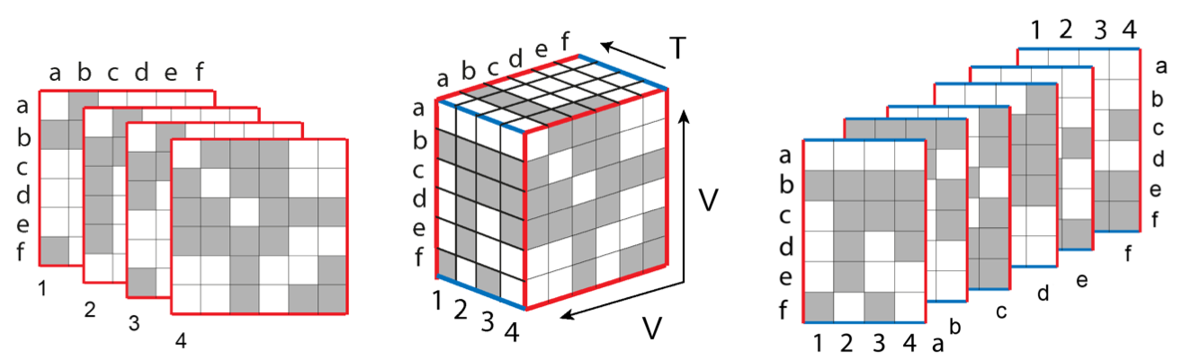
Figure 1: Matrix cube (center) with Time slices (left) and Vertex slices (right).
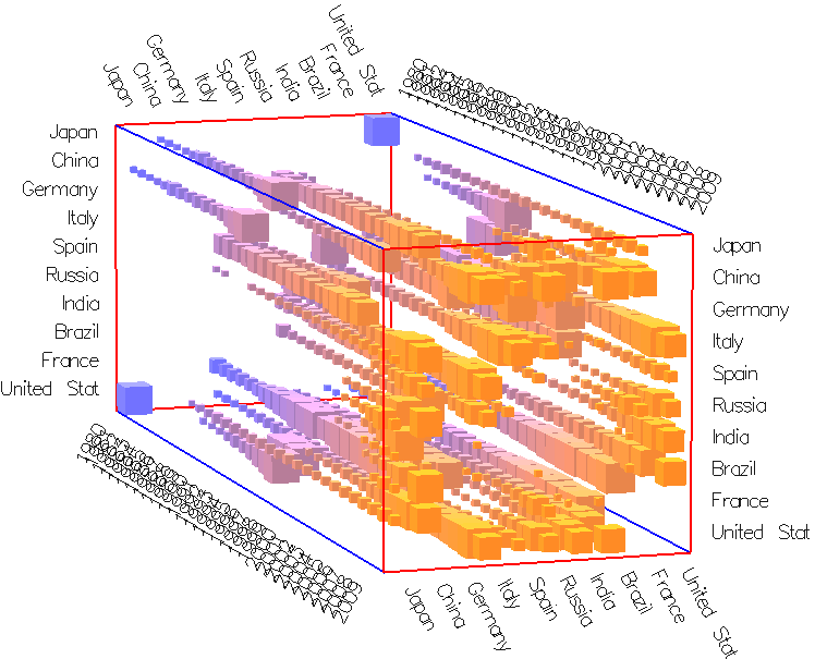
The cube also can exhibit vectors (Figure 2) which either show the evolution of connectivity of an individual node pair (blue), or the node's neighborhood at a given time point (red).
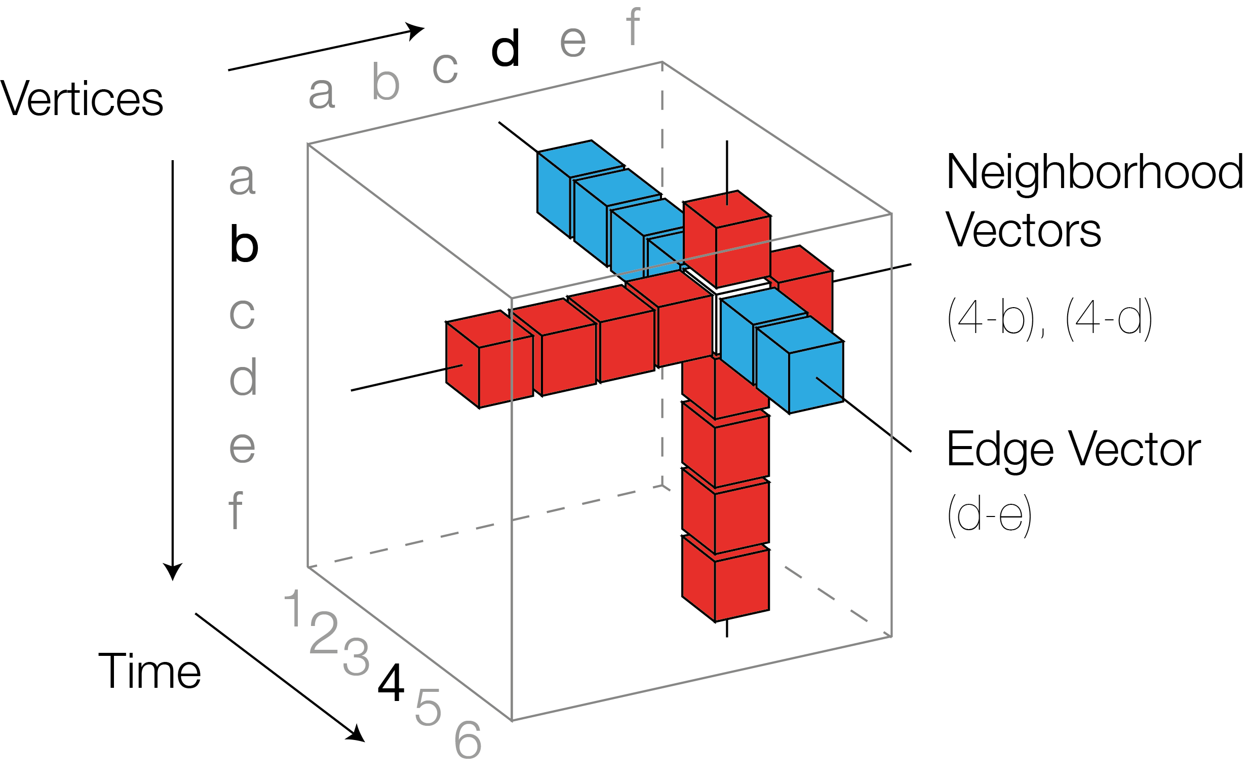
Figure 2:Vectors in the Matrix Cube
Cubix Interface
Visualization an exploration of three-dimensional models on the screen is difficult. With Cubix, we provide transformation and decomposition operations which yield better readable 2D representations of the information contained in the cube.
The interface of Cubix, with the cube as main component is shown in Figure 3.
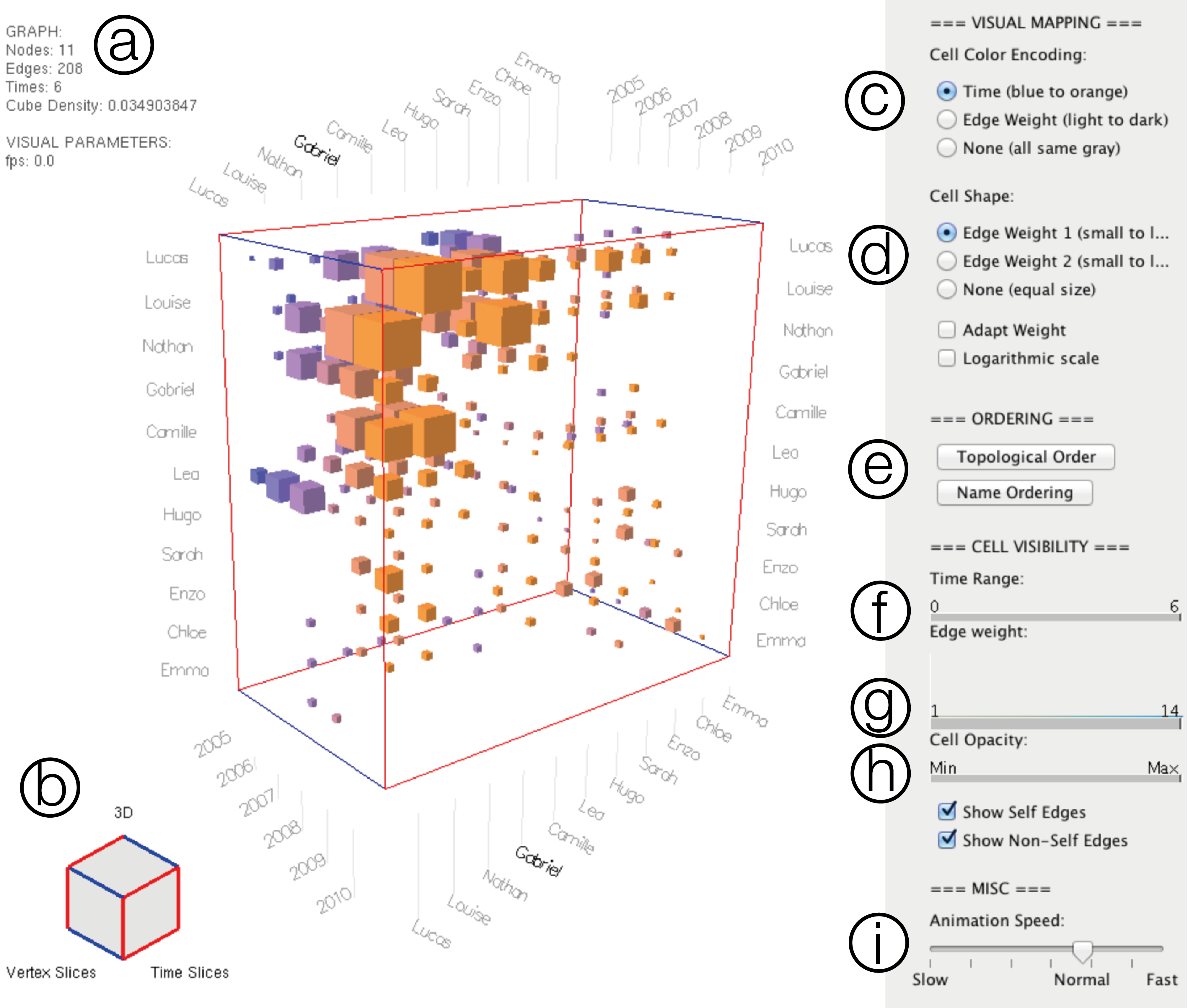
Figure 3:Screenshot from Cubix interface with the following components:
- a) Some network statistics,
- b) Cubelet Widget,
- c) Cell color encoding,
- d) Cell shape encoding,
- e) Vertex ordering options,
- f) Time range slider,
- g) Cell weight slider,
- h) Cell opacity slider,
- i) Animation speed slider.
Views
Cubix implements several prefefined views on the (decomposed) Matrix Cube. The views in Cubix are summarized in the following figure:
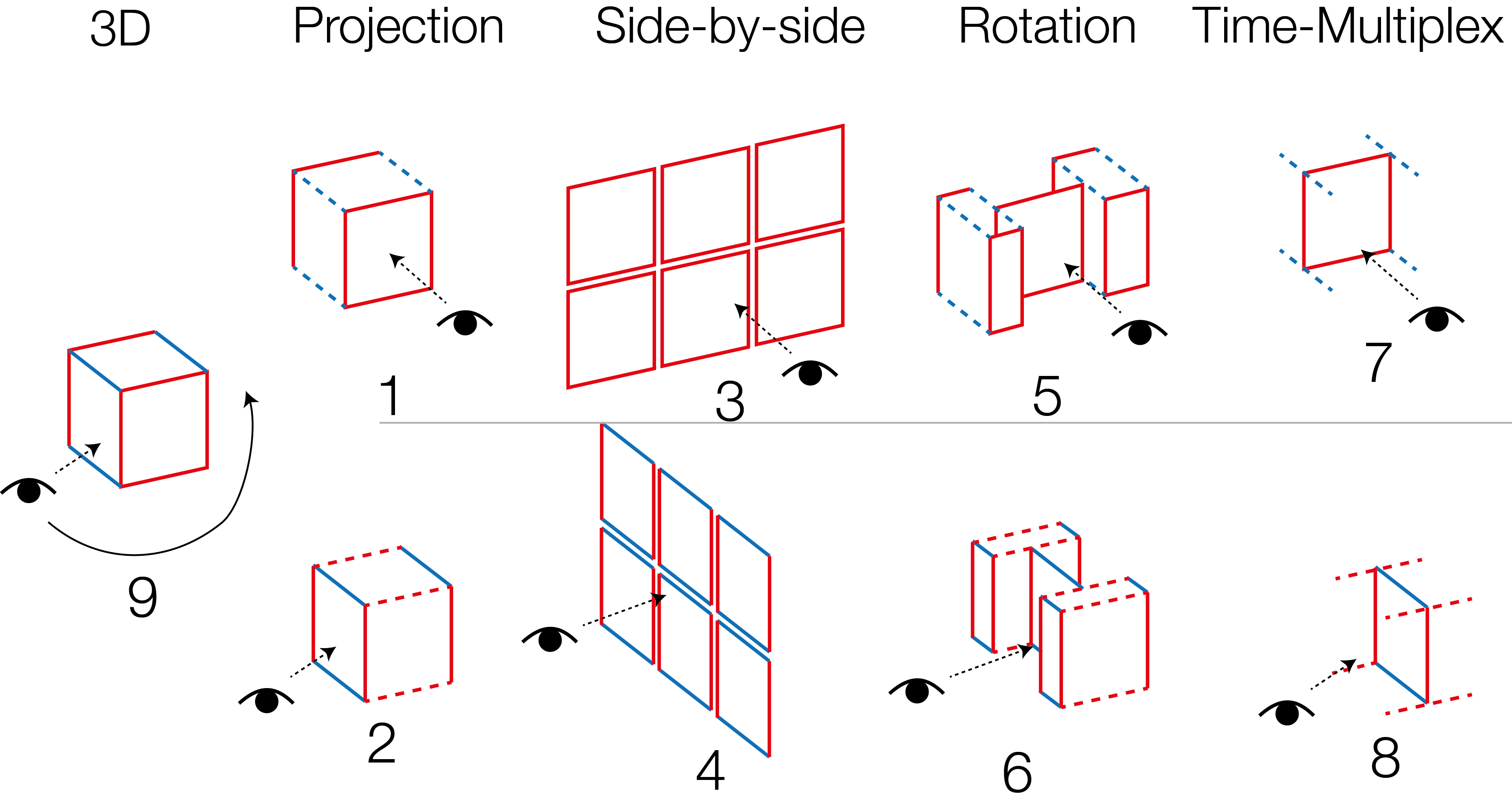
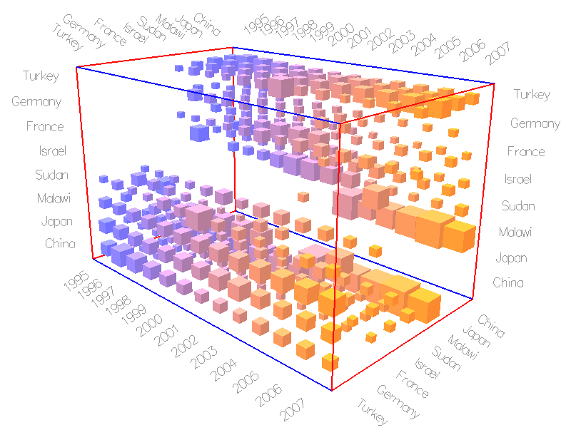
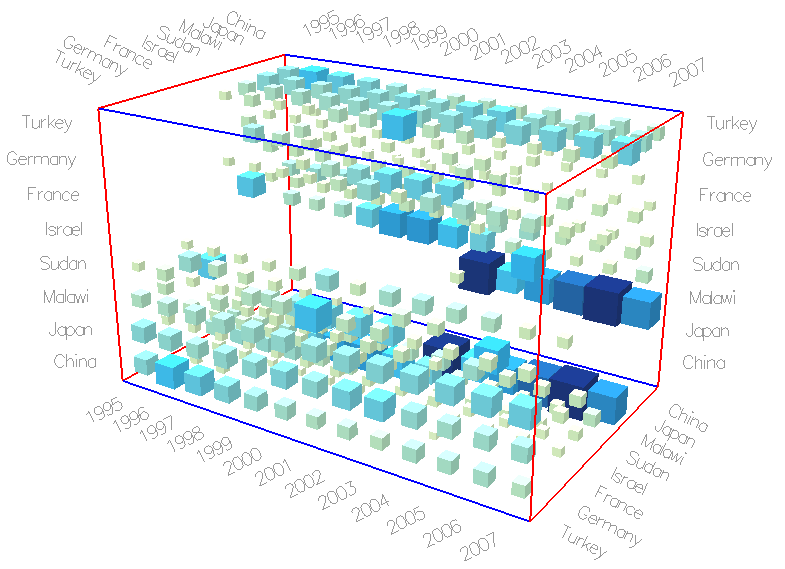
3D and Projection
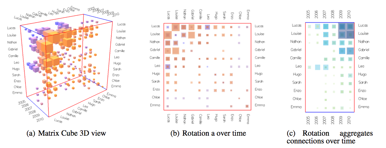
Figure 3: 3D view, Front projection and side projection.
While the 3D view offers a quick overview (Figure 3a) of the dynamic network, projecting the cube orthogonally, yields aggregated views.
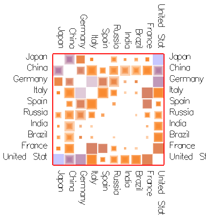
The front projection (Figure 3b) shows a summary of the connections between any node pair. The front view can show clusters and outliers in the network's topology.
The side projection (Figure 3c) shows a summary of the connectedness (activity) of each node over time and can reveal general trends about network density.
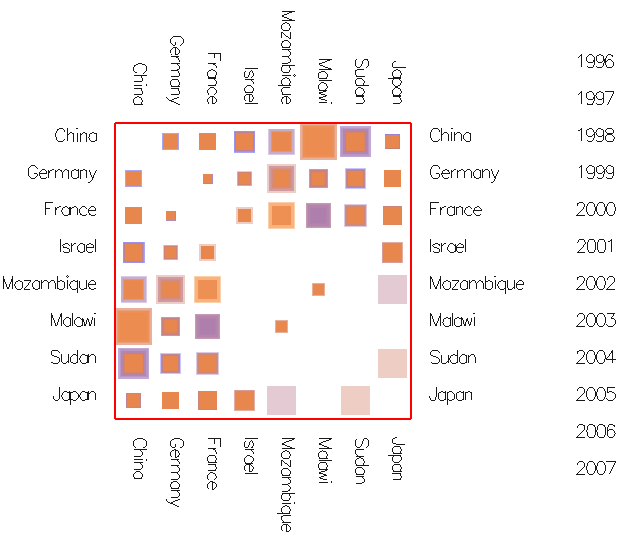
Rotated Slices
While the cube is projected, slices can be rotated to face the user, like books in a bookshelf (Figures 4 and 5). gRotating a slice allows detailed view on the slice, while maintaining an aggregated view of the cube around.
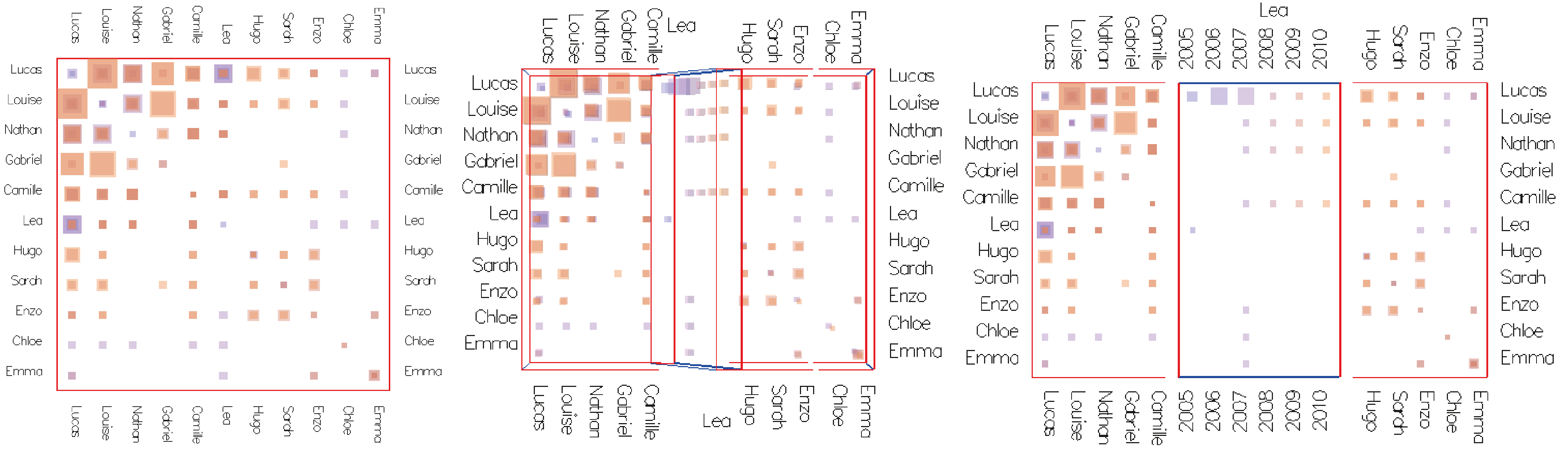
Figure 4: Vertex slice rotated
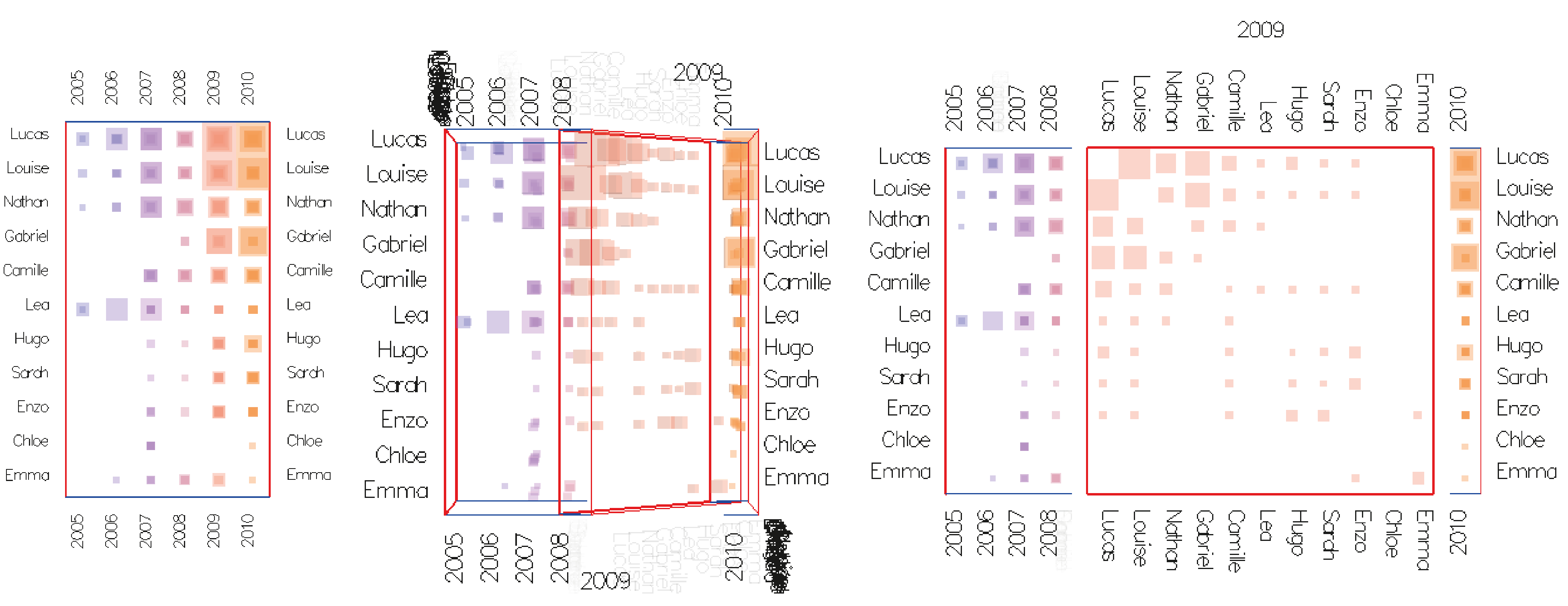
Figure 5: Time slice rotated.
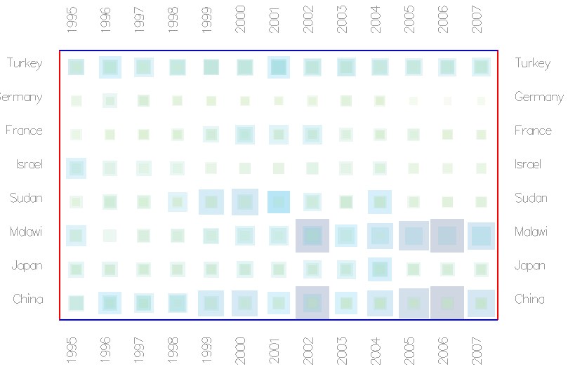
Small Multiples
A simple mouse click in Cubix lays out all time or vertex slices side-by-side on the screen. The user can freely pan and zoom.
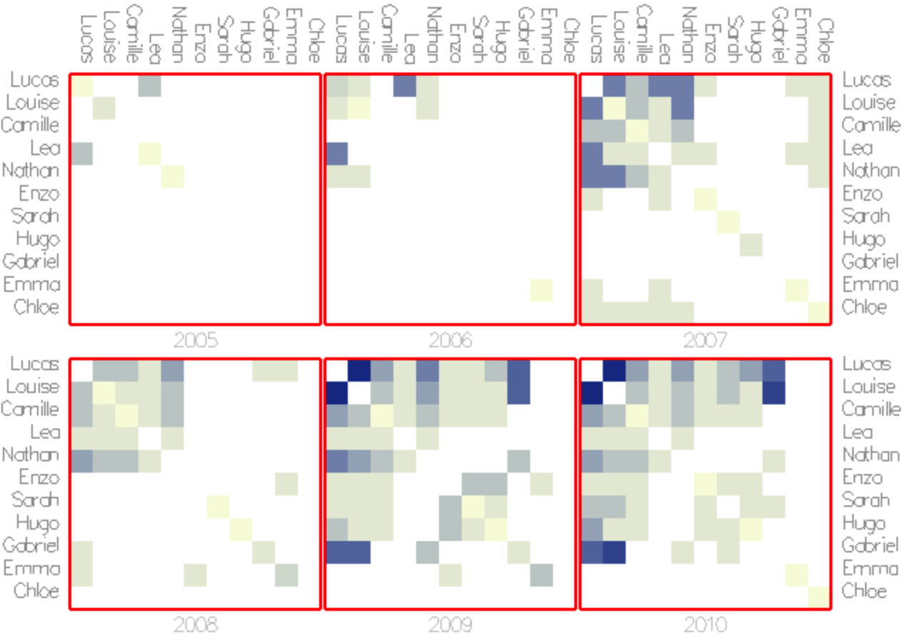
Figure 6: Time slices (adjacency matrices) side by side. Blue cells indicate connections with high weight values, beige cells indicate connections with small edge weights. This view gives an overview of all time steps at a glance and to a certain extend allows comparison.
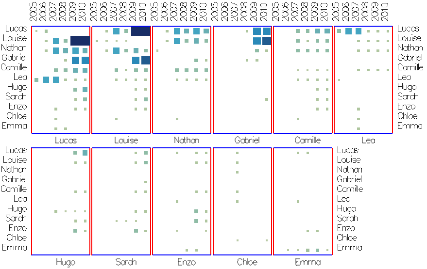
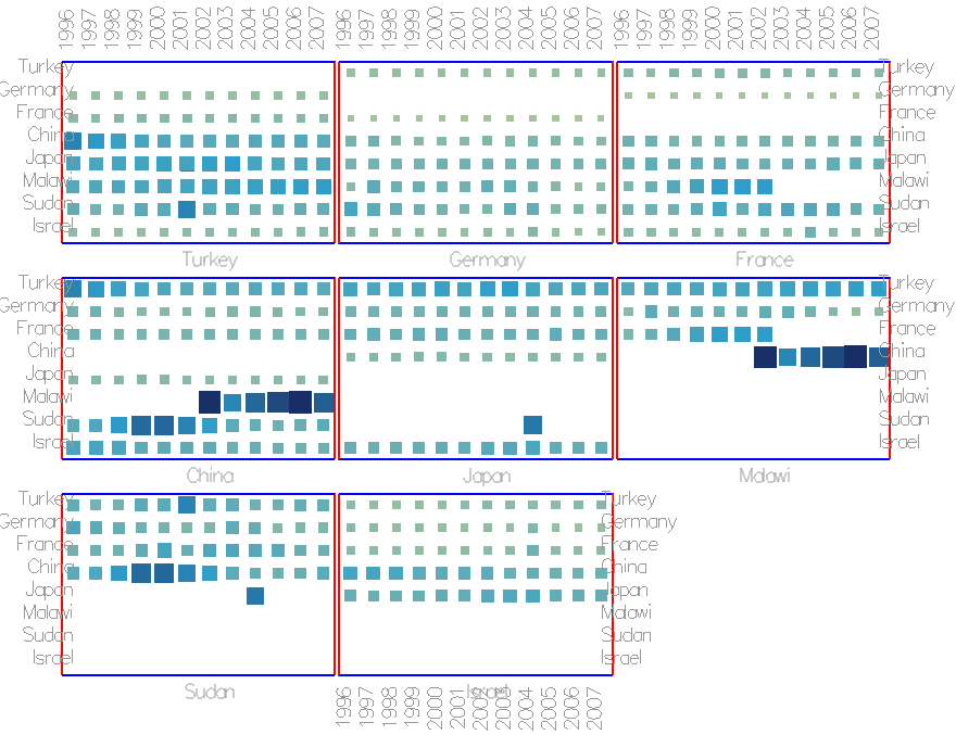
Figure 7: Vertex slices side-by-side. This view gives an overview of how different nodes (persons, countries, etc) behave in the network and what connection patterns exist.
Flip Book
Besides small multiples, individual slices can be selected and observed individually. Using the arrow keys, users can flip though all time or vertex slices similar to a power-point presentation.
View Navigation with Cubelet
Switching between views is facilitated by the Cubelet Widget, shown in Figure 8. Each face of the Cubelet, in conjunction with a mouse gesture corresponds to a predefined view in Cubix. Switching between views happens though animated transitions.
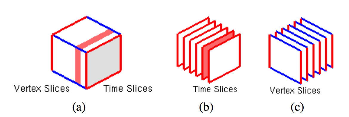
Figure 8: Cubelet widget for rapid navigation.
Further Exploration Features
- Visual Encoding -- Users can chose among three different color encodings for cells and three encodings for cell shape. Each encoding shows a different aspect of the data.
- Filtering --- To decrease density of the cube, edges can be filtered (removed from display) according to time, vertices and/or weight.
- Reorder rows and columns -- Rows and columns in the cube can be reordered at any time, taking only the visible cells into account. Automatically reordering rows and columns in the cube shows patterns in the data, such as clusters and outliers.
Examples
Trading volume between countries
 |
 Trading costs between countries |
 |
 |
 |
 |
 |